Tables - Part II
This is only available in the Pro-version of the library.
In Part I of this serie we showed the basic principle of working with tables and what basic APIs was available. In this second part we will show some case studies on how to use this to achieve some nice looking graphs. This is a living document and new case studies will be added in the future.
Case study 1 - Aligning a table just below a graph
The goal of this example is to explain in detail how to achieve the graphs shown in Figure 1.
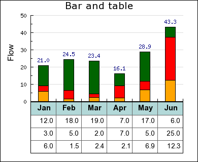
Figure 1. Illustrating data with both a graph and a table.
The graph in figure 1 consists of a standard accumulated bar graph combined with a table just below the X-axis. The way to create such a graph is very basic. First create a standard bar graph with some extra bottom margin (to make room for the table) and then create and position the table below the graph. The only slightly tricy is to make sure that the width of the table and graph matches to line up each column under each bar. Lets walk through the steps to do this.
The data to be plotted in the bar and in the table is created in a table as follows
$datay = array(
    array('Jan','Feb','Mar','Apr','May','Jun'),
    array(12,18,19,7,17,6),
    array(3,5,2,7,5,25),
    array(6,1.5,2.4,2.1,6.9,12.3));
each line in this matrix corresponds to one row in the table and one set of bars that will make up the accumulated bar plot.
First let's define some constants that will control the size and positoin of the graph and table.
$nbrbar = 6; // number of bars and hence number of columns in table
$cellwidth = 50;  // width of each column in the table
$tableypos = 200; // top left Y-coordinate for table
$tablexpos = 60;  // top left X-coordinate for table
$tablewidth = $nbrbar*$cellwidth; // overall table width
$rightmargin = 30;  // right margin in the graph
$topmargin = 30  // top margin of graph
The next step is to calculate a suitable size for the entire graph, i.e. the entire image.
$height = 320;  // a suitable height for the image
$width = $tablexpos+$tablewidth+$rightmargin; // the width of the image
Finally its time ot make use of these constants to rceate the basic graph. Note that we calculate the bottom margin to just fit the tables selected Y-coordinate position.
$graph = new Graph($width,$height);
$graph->img->SetMargin($tablexpos,$rightmargin,$topmargin,$height-$tableypos);
$graph->SetScale('textlin');
$graph->SetMarginColor('white');
The rest of the code to create the accumulated bar plot is pretty mundane and we just show the code here without further comment.
// Create the bars and the accbar plot
$bplot = new BarPlot($datay[3]);
$bplot->SetFillColor('orange');
$bplot2 = new BarPlot($datay[2]);
$bplot2->SetFillColor('red');
$bplot3 = new BarPlot($datay[1]);
$bplot3->SetFillColor('darkgreen');
$accbplot = new AccBarPlot(array($bplot,$bplot2,$bplot3));
$accbplot->value->Show();
$graph->Add($accbplot);
It's now time to setup the table. The position of the table is determined by the previous set constants and the original data as specified above.
$table = new GTextTable();
$table->Set($datay);
$table->SetPos($tablexpos,$tableypos+1);
The rest of the table formatting is fairly basic and again we just show the necessary script without further comment.
$table->SetFont(FF_ARIAL,FS_NORMAL,10);
$table->SetAlign('right');
$table->SetMinColWidth($cellwidth);
$table->SetNumberFormat('%0.1f');

// Format table header row
$table->SetRowFillColor(0,'teal@0.7');
$table->SetRowFont(0,FF_ARIAL,FS_BOLD,11);
$table->SetRowAlign(0,'center');

// .. and add it to the graph
$graph->Add($table);